Data Visualization in Python with matplotlib andSeaborn

Data visualization is an important aspect of all AI and machine learning applications. You can gain key insights of your data through different graphical representations. In this tutorial, we’ll talk about a few options for data visualization in Python. We’ll use the MNIST dataset and the Tensorflow library for number crunching and data manipulation. To illustrate various methods for creating different types of graphs, we’ll use the Python’s graphing libraries namely matplotlib, Seaborn

After completing this tutorial, you will know:

• How to visualize images in matplotlib
• How to make scatter plots in matplotlib, Seaborn 
• How to make multiline plots in matplotlib, Seaborn 

Let’s get started.

Preparation of scatter data

In this post, we will use matplotlib, seaborn, and bokeh. They are all external libraries need to be installed. To install them using pip, run the following command:

1	pip install matplotlib seaborn bokeh

For demonstration purposes, we will also use the MNIST handwritten digits dataset. We will load it from Tensorflow and run PCA algorithm on it. Hence we will also need to install Tensorflow and pandas:

1	pip install tensorflow pandas

The code afterwards will assume the following imports are executed:

1 2 3 4 5 6 7 8 9 10 11 12 13 14 15 16 17 18

# Importing from tensorflow and keras from tensorflow.keras.datasets import mnist from tensorflow.keras.models import Sequential from tensorflow.keras.layers import Dense, Reshape from tensorflow.keras import utils from tensorflow import dtypes, tensordot from tensorflow import convert_to_tensor, linalg, transpose # For math operations import numpy as np # For plotting with matplotlib import matplotlib.pyplot as plt # For plotting with seaborn import seaborn as sns   # For plotting with bokeh from bokeh.plotting import figure, show from bokeh.models import Legend, LegendItem # For pandas dataframe import pandas as pd

We load the MNIST dataset from keras.datasets library. To keep things simple, we’ll retain only the subset of data containing the first three digits. We’ll also ignore the test set for now.

1 2 3 4 5 6 7 8 9 10 11 12

... # load dataset (x_train, train_labels), (_, _) = mnist.load_data() # Choose only the digits 0, 1, 2 total_classes = 3 ind = np.where(train_labels < total_classes) x_train, train_labels = x_train[ind], train_labels[ind] # Shape of training data total_examples, img_length, img_width = x_train.shape # Print the statistics print('Training data has ', total_examples, 'images') print('Each image is of size ', img_length, 'x', img_width)

1 2	Training data has  18623 images Each image is of size  28 x 28

Figures in matplotlib

Seaborn is indeed an add-on to matplotlib. Therefore you need to understand how matplotlib handles plots even if you’re using Seaborn.

Matplotlib calls its canvas the figure. You can divide the figure into several sections called subplots, so you can put two visualizations side-by-side.

As an example, let’s visualize the first 16 images of our MNIST dataset using matplotlib. We’ll create 2 rows and 8 columns using the subplots() function. The subplots() function will create the axes objects for each unit. Then we will display each image on each axes object using the imshow() method. Finally, the figure will be shown using the show() function.

1 2 3 4 5 6 7 8

img_per_row = 8 fig,ax = plt.subplots(nrows=2, ncols=img_per_row,                       figsize=(18,4),                       subplot_kw=dict(xticks=[], yticks=[])) for row in [0, 1]:     for col in range(img_per_row):         ax[row, col].imshow(x_train[row*img_per_row + col].astype('int'))   plt.show()

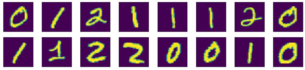
First 16 images of the training dataset displayed in 2 rows and 8 columns

Here we can see a few properties of matplotlib. There is a default figure and default axes in matplotlib. There are a number of functions defined in matplotlib under the pyplot submodule for plotting on the default axes. If we want to plot on a particular axes, we can use the plotting function under the axes objects. The operations to manipulate a figure is procedural. Meaning, there is a data structure remembered internally by matplotlib and our operations will mutate it. The show() function simply display the result of a series of operations. Because of that, we can gradually fine-tune a lot of details on the figure. In the example above, we hid the “ticks” (i.e., the markers on axes) by setting xticks and yticks to empty lists.

Scatter plots in matplotlib and Seaborn

One of the common visualizations we use in machine learning projects is the scatter plot.

As an example, we apply PCA to the MNIST dataset and extract the first three components of each image. In the code below, we compute the eigenvectors and eigenvalues from the dataset, then projects the data of each image along the direction of the eigenvectors, and store the result in x_pca. For simplicity, we didn’t normalize the data to zero mean and unit variance before computing the eigenvectors. This omission does not affect our purpose of visualization.

1 2 3 4 5 6 7 8 9 10

... # Convert the dataset into a 2D array of shape 18623 x 784 x = convert_to_tensor(np.reshape(x_train, (x_train.shape[0], -1)),                       dtype=dtypes.float32) # Eigen-decomposition from a 784 x 784 matrix eigenvalues, eigenvectors = linalg.eigh(tensordot(transpose(x), x, axes=1)) # Print the three largest eigenvalues print('3 largest eigenvalues: ', eigenvalues[-3:]) # Project the data to eigenvectors x_pca = tensordot(x, eigenvectors, axes=1)

The eigenvalues printed are as follows:

1	3 largest eigenvalues:  tf.Tensor([5.1999642e+09 1.1419439e+10 4.8231231e+10], shape=(3,), dtype=float32)

The array x_pca is in shape 18623 x 784. Let’s consider the last two columns as the x- and y-coordinates and make the point of each row in the plot. We can further color the point according to which digit it corresponds to.

The following code generates a scatter plot using matplotlib. The plot is created using the axes object’s scatter() function, which takes the x- and y-coordinates as the first two argument. The c argument to scatter() method specifies a value that will become its color. The s argument specifies its size. The code also creates a legend and adds a title to the plot.

1 2 3 4 5 6 7

fig, ax = plt.subplots(figsize=(12, 8)) scatter = ax.scatter(x_pca[:, -1], x_pca[:, -2], c=train_labels, s=5) legend_plt = ax.legend(*scatter.legend_elements(),                        loc="lower left", title="Digits") ax.add_artist(legend_plt) plt.title('First Two Dimensions of Projected Data After Applying PCA') plt.show()

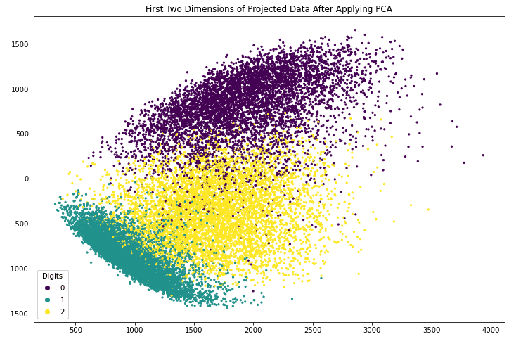
2D scatter plot generated using matplotlib

Putting the above altogether, the following is the complete code to generate the 2D scatter plot using matplotlib:

1 2 3 4 5 6 7 8 9 10 11 12 13 14 15 16 17 18 19 20 21 22 23 24 25 26 27 28 29 30 31 32 33 34 35

from tensorflow.keras.datasets import mnist from tensorflow import dtypes, tensordot from tensorflow import convert_to_tensor, linalg, transpose import numpy as np import matplotlib.pyplot as plt   # Load dataset (x_train, train_labels), (_, _) = mnist.load_data() # Choose only the digits 0, 1, 2 total_classes = 3 ind = np.where(train_labels < total_classes) x_train, train_labels = x_train[ind], train_labels[ind] # Verify the shape of training data total_examples, img_length, img_width = x_train.shape print('Training data has ', total_examples, 'images') print('Each image is of size ', img_length, 'x', img_width)   # Convert the dataset into a 2D array of shape 18623 x 784 x = convert_to_tensor(np.reshape(x_train, (x_train.shape[0], -1)),                       dtype=dtypes.float32) # Eigen-decomposition from a 784 x 784 matrix eigenvalues, eigenvectors = linalg.eigh(tensordot(transpose(x), x, axes=1)) # Print the three largest eigenvalues print('3 largest eigenvalues: ', eigenvalues[-3:]) # Project the data to eigenvectors x_pca = tensordot(x, eigenvectors, axes=1)   # Create the plot fig, ax = plt.subplots(figsize=(12, 8)) scatter = ax.scatter(x_pca[:, -1], x_pca[:, -2], c=train_labels, s=5) legend_plt = ax.legend(*scatter.legend_elements(),                        loc="lower left", title="Digits") ax.add_artist(legend_plt) plt.title('First Two Dimensions of Projected Data After Applying PCA') plt.show()

Matplotlib also allows a 3D scatter plot to be produced. To do so, you need to create an axes object with 3D projection first. Then the 3D scatter plot is created with the scatter3D() function, with the x-, y-, and z-coordinates as the first three arguments. The code below uses the data projected along the eigenvectors corresponding to the three largest eigenvalues. Instead of creating a legend, this code creates a colorbar.

1 2 3 4 5

fig = plt.figure(figsize=(12, 8)) ax = plt.axes(projection='3d') plt_3d = ax.scatter3D(x_pca[:, -1], x_pca[:, -2], x_pca[:, -3], c=train_labels, s=1) plt.colorbar(plt_3d) plt.show()

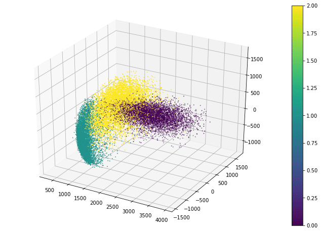
3D scatter plot generated using matplotlib

The scatter3D() function just puts the points onto the 3D space. Afterwards, we can still modify how the figure displays such as the label of each axis and the background color. But in 3D plots, one common tweak is the viewport, namely, the angle we look at the 3D space. Viewport is controlled by the view_init() function in the axes object:

1	ax.view_init(elev=30, azim=-60)

The viewport is controlled by the elevation angle (i.e., angle to the horizon plane) and the azimuthal angle (i.e., rotation on the horizon plane). By default, matplotlib uses 30 degree elevation and -60 degree azimuthal, as shown above.

Putting everything together, the following is the complete code to create the 3D scatter plot in matplotlib:

1 2 3 4 5 6 7 8 9 10 11 12 13 14 15 16 17 18 19 20 21 22 23 24 25 26 27 28 29 30 31 32 33 34

from tensorflow.keras.datasets import mnist from tensorflow import dtypes, tensordot from tensorflow import convert_to_tensor, linalg, transpose import numpy as np import matplotlib.pyplot as plt   # Load dataset (x_train, train_labels), (_, _) = mnist.load_data() # Choose only the digits 0, 1, 2 total_classes = 3 ind = np.where(train_labels < total_classes) x_train, train_labels = x_train[ind], train_labels[ind] # Verify the shape of training data total_examples, img_length, img_width = x_train.shape print('Training data has ', total_examples, 'images') print('Each image is of size ', img_length, 'x', img_width)   # Convert the dataset into a 2D array of shape 18623 x 784 x = convert_to_tensor(np.reshape(x_train, (x_train.shape[0], -1)),                       dtype=dtypes.float32) # Eigen-decomposition from a 784 x 784 matrix eigenvalues, eigenvectors = linalg.eigh(tensordot(transpose(x), x, axes=1)) # Print the three largest eigenvalues print('3 largest eigenvalues: ', eigenvalues[-3:]) # Project the data to eigenvectors x_pca = tensordot(x, eigenvectors, axes=1)   # Create the plot fig = plt.figure(figsize=(12, 8)) ax = plt.axes(projection='3d') ax.view_init(elev=30, azim=-60) plt_3d = ax.scatter3D(x_pca[:, -1], x_pca[:, -2], x_pca[:, -3], c=train_labels, s=1) plt.colorbar(plt_3d) plt.show()

Creating scatter plots in Seaborn is similarly easy. The scatterplot() method automatically creates a legend and uses different symbols for different classes when plotting the points. By default, the plot is created on the “current axes” from matplotlib, unless the axes object is specified by the ax argument.

1 2 3 4 5 6

fig, ax = plt.subplots(figsize=(12, 8)) sns.scatterplot(x_pca[:, -1], x_pca[:, -2],                 style=train_labels, hue=train_labels,                 palette=["red", "green", "blue"]) plt.title('First Two Dimensions of Projected Data After Applying PCA') plt.show()

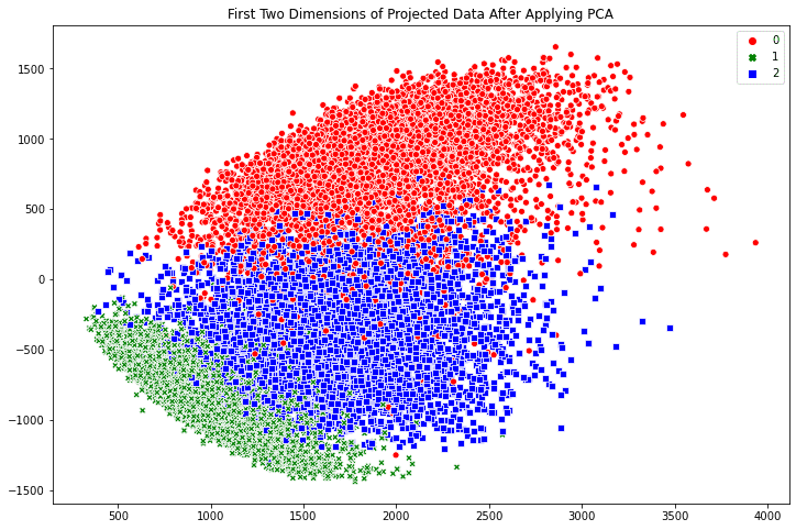
2D scatter plot generated using Seaborn

The benefit of Seaborn over matplotlib is two fold: First we have a polished default style. For example, if we compare the point style in the two scatter plots above, the Seaborn one has a border around the dot to prevent the many points smurged together. Indeed, if we run the following line before calling any matplotlib functions:

1	sns.set(style = "darkgrid")

we can still use the matplotlib functions but get a better looking figure by using Seaborn’s style. Secondly, it is more convenient to use Seaborn if we are using pandas DataFrame to hold our data. As an example, let’s convert our MNIST data from a tensor into a pandas DataFrame:

1 2 3

df_mnist = pd.DataFrame(x_pca[:, -3:].numpy(), columns=["pca3","pca2","pca1"]) df_mnist["label"] = train_labels print(df_mnist)

which the DataFrame looks like the following:

1 2 3 4 5 6 7 8 9 10 11 12 13 14

pca3        pca2         pca1  label 0     -537.730103  926.885254  1965.881592      0 1      167.375885 -947.360107  1070.359375      1 2      553.685425 -163.121826  1754.754272      2 3     -642.905579 -767.283020  1053.937988      1 4     -651.812988 -586.034424   662.468201      1 ...           ...         ...          ...    ... 18618  415.358948 -645.245972   853.439209      1 18619  754.555786    7.873116  1897.690552      2 18620 -321.809357  665.038086  1840.480225      0 18621  643.843628  -85.524895  1113.795166      2 18622   94.964279 -549.570984   561.743042      1   [18623 rows x 4 columns]

Then, we can reproduce the Seaborn’s scatter plot with the following:

1 2 3 4 5 6

fig, ax = plt.subplots(figsize=(12, 8)) sns.scatterplot(data=df_mnist, x="pca1", y="pca2",                 style="label", hue="label",                 palette=["red", "green", "blue"]) plt.title('First Two Dimensions of Projected Data After Applying PCA') plt.show()

which we do not pass in arrays as coordinates to the scatterplot() function, but column names to the data argument instead.

The following is the complete code to generate a scatter plot using Seaborn with the data stored in pandas:

1 2 3 4 5 6 7 8 9 10 11 12 13 14 15 16 17 18 19 20 21 22 23 24 25 26 27 28 29 30 31 32 33 34 35 36 37 38 39 40

from tensorflow.keras.datasets import mnist from tensorflow import dtypes, tensordot from tensorflow import convert_to_tensor, linalg, transpose import numpy as np import pandas as pd import matplotlib.pyplot as plt import seaborn as sns   # Load dataset (x_train, train_labels), (_, _) = mnist.load_data() # Choose only the digits 0, 1, 2 total_classes = 3 ind = np.where(train_labels < total_classes) x_train, train_labels = x_train[ind], train_labels[ind] # Verify the shape of training data total_examples, img_length, img_width = x_train.shape print('Training data has ', total_examples, 'images') print('Each image is of size ', img_length, 'x', img_width)   # Convert the dataset into a 2D array of shape 18623 x 784 x = convert_to_tensor(np.reshape(x_train, (x_train.shape[0], -1)),                       dtype=dtypes.float32) # Eigen-decomposition from a 784 x 784 matrix eigenvalues, eigenvectors = linalg.eigh(tensordot(transpose(x), x, axes=1)) # Print the three largest eigenvalues print('3 largest eigenvalues: ', eigenvalues[-3:]) # Project the data to eigenvectors x_pca = tensordot(x, eigenvectors, axes=1)   # Making pandas DataFrame df_mnist = pd.DataFrame(x_pca[:, -3:].numpy(), columns=["pca3","pca2","pca1"]) df_mnist["label"] = train_labels   # Create the plot fig, ax = plt.subplots(figsize=(12, 8)) sns.scatterplot(data=df_mnist, x="pca1", y="pca2",                 style="label", hue="label",                 palette=["red", "green", "blue"]) plt.title('First Two Dimensions of Projected Data After Applying PCA') plt.show()

Seaborn as a wrapper to some matplotlib functions, is not replacing matplotlib entirely. Plotting in 3D, for example, are not supported by Seaborn and we still need to resort to matplotlib functions for such purposes.